CASE87 · District heating · Weather-adaptive control
Weather-adaptive supply-temperature guidance for district-heated apartments
A historical-weather simulation compares conventional outdoor-air reset with an hourly demand-aware supply-temperature guide. The outputs describe setpoint differences and improvement potential, not measured heat savings.
01 · CASE ANALYSIS
Case question
How much can a recommended supply temperature change when hourly heating-demand patterns are included alongside outdoor temperature? What field M&V would be required to demonstrate actual savings?
The program compares a conventional outdoor-temperature-based reset setting with a smart guide incorporating hourly heating demand and heating degree hours (HDH). Both operate within a 43–50°C supply-temperature range.
02 · CASE ANALYSIS
Simulation method
Obtain hourly Seoul temperatures, select the winter periods, calculate the conventional reset setpoint and the demand-aware recommendation for the same hours, and aggregate the differences.
This calculation uses historical observations, not a verified live forecast-control deployment. A forecast connection is a possible subsequent step. Site calibration must precede use of the recommendations in actual operation.
| Indicator | Reported value |
|---|---|
| Hourly weather observations | 8,760 records; Seoul, 2023 |
| Winter analysis hours | 3,624 h |
| Supply-temperature range | 43–50°C |
| Conventional reset mean | 46.785°C |
| Smart-guide mean | 46.034°C |
| Mean difference | 0.751°C |
| Hours with a lower smart recommendation | Approximately 88.6% |
03 · CASE ANALYSIS
Reported results
Across 3,624 winter hours, the mean conventional reset setting was 46.785°C and the mean smart recommendation 46.034°C. The average difference was 0.751°C.
The smart guide recommended a lower supply temperature for approximately 88.6% of the analyzed hours. These are setpoint outputs; they do not establish a heat-energy savings percentage.
Dividing the mean temperature difference by the 7°C control range must not be presented as an energy-saving rate.
04 · CASE ANALYSIS
Field application & calibration
The guide could help mechanical-room operators review early-morning settings and avoid excess supply. BAS/BEMS could display recommendations or apply them automatically after appropriate commissioning.
Calibrate supply limits, hourly demand patterns, outdoor-temperature influence and acceptable complaint levels for each complex. Use several weeks of supply/return temperatures, indoor temperatures, heat-meter readings and complaint records.
05 · CASE ANALYSIS
Measurement & verification
Assess whether actual heat use falls while equivalent service is maintained. Compare adjusted baseline heat use with actual heat use within the same measurement boundary, using HDD and relevant operating conditions.
Verified saving = adjusted baseline heat use − actual heat use. Keep this future field-verification result distinct from the simulation’s temperature difference.
Source figures · English edition
Figures correspond to those published in the Korean case. English titles, axes and legends are provided; published values and evidence boundaries are retained. Open a figure at full size to inspect small labels.
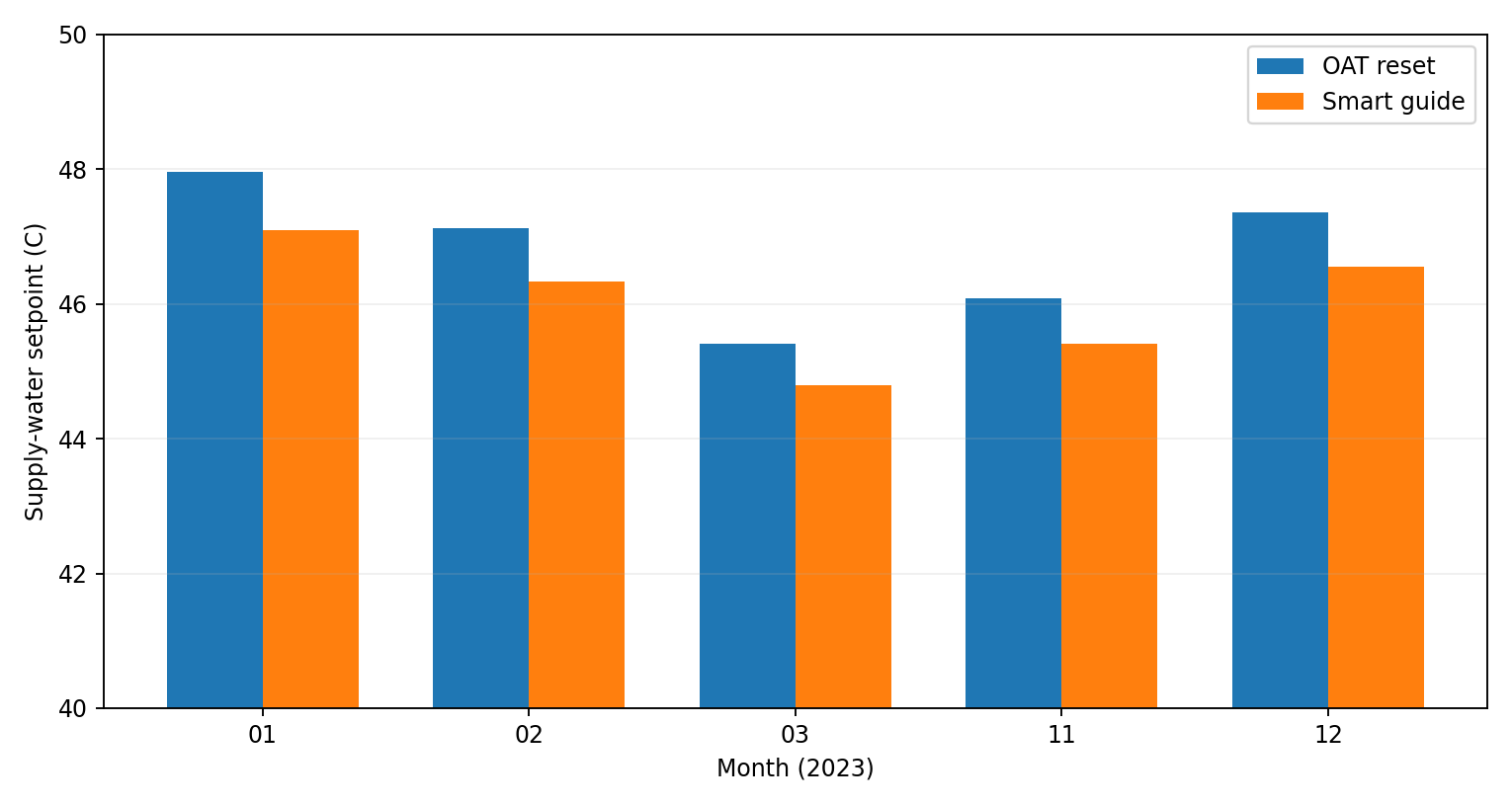
Original already-English monthly supply-temperature comparison for the 2023 weather simulation. Setpoint reductions are not measured heating-energy savings.
Open full-size figure ↗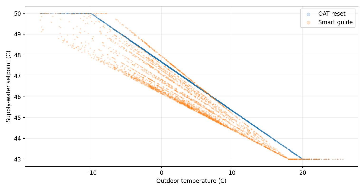
Original already-English setpoint curves/scatter against outdoor temperature. Historical model outputs with the source limits preserved.
Open full-size figure ↗APPLY TO YOUR SITE
Connect your operating data to an actionable energy strategy.
Discuss the measurement boundary, data quality, operating constraints and verification approach for your facility.
Discuss your project All English cases